Constructing an HNSW Graph（Lucene 9.8.0）

Lucene has implemented the HNSW (Hierarchical Navigable Small World) logic based on the paper ‘Efficient and robust approximate nearest neighbor search using Hierarchical Navigable Small World graphs [2018].’ This article, in conjunction with the Lucene source code, introduces the implementation details during the construction process.

Overview

Figure 1：

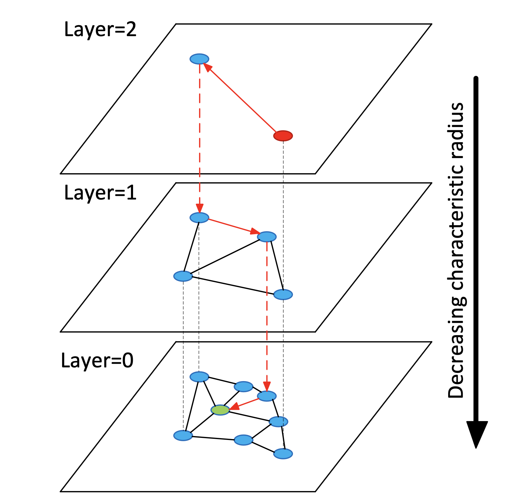
Let’s first introduce some basic knowledge about the completed HNSW (Hierarchical Navigable Small World) graph, briefly explained through Figure 1 from the paper:

1. Hierarchical Structure: The HNSW graph has a multi-layered structure, where each layer is an independent graph. The number of layers is usually determined based on the size and complexity of the dataset. At the top layer (as shown in Figure 1 as layer=2), there are fewer nodes, but each node covers a broader range. Conversely, at the bottom layer (layer=0), there are more nodes, but each node covers a relatively smaller area.
2. Node Connections: In each layer, nodes are connected to their neighbors through edges. These connections are based on distance or similarity metrics, meaning each node tends to connect with other nodes closest to it.
3. Neighbor Selection: The choice of which nodes to consider as neighbors is based on certain heuristic rules aimed at balancing search efficiency and accuracy. Typically, this involves maintaining the diversityof neighbors and limiting the number of neighbors for each node.
4. Search Path: Both the construction and querying of the HNSW graph involve a search process. The search path starts from a global entry node at the highest layer and then descends layer by layer until reaching the bottom layer. In each layer, the search follows the layer’s connection structure to find nodes closest to the target node.

Implementation

To introduce the construction of the HNSW graph in Lucene, we will explain it through the process of adding/inserting a new node:

Figure 2：

New Node

Figure 3：

In Lucene, each Document can only have one vector with the same field name, and each vector is assigned a node identifier (nodeId) in the order they are added. This nodeId is a value that starts from 0 and increases incrementally. In the source code, the new node is represented by this nodeId. When we need to calculate the distance between two nodes, we can find the corresponding vector values of the nodes through this mapping relationship for calculation.

Calculating the Target Level

Figure 4：

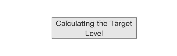
The target level is calculated as a random number that follows an exponential distribution.

The HNSW graph has a multi-layered structure, and the target level determines in which layers the new node will be added and establish connections with other nodes.

For example, if the target level is 3, then the node will be added to layers 3, 2, 1, and 0, respectively.

Calculation Formula

In the source code, the target level is calculated using the formula: -ln(unif(0,1)) * ml, where unif(0,1) represents a uniformly distributed random value between 0 and 1, and ml is defined as 1/ln(M), where M(defined in source code as maxConn) is the maximum number of connections, i.e., a node can connect with up to M other nodes(2*M at the bottom). In the source code, the default value for M is 16.

The theoretical and experimental basis for using this formula is detailed in the paper; this article does not elaborate on it.

Are There Any Unprocessed Levels Remaining?

Figure 5：

After calculating the target level, the process starts from the highest level and works downwards, layer by layer, until the new node is added to all levels and connections with other nodes are established. This completes the insertion of the new node.

Retrieving the Entry Node

Figure 6：

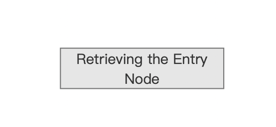
An entry point is a starting point that guides the insertion of a new node into a certain layer (there may be multiple entry points, as described below).

The purpose of inserting a new node into a layer is to establish its connections with other nodes in that layer. Therefore, on one hand, it first connects with the entry node, and on the other hand, it tries to establish connections with the neighbors of the entry node, the neighbors of the neighbors of the entry node, and so on, based on a greedy algorithm. This process will be detailed in the flow point Identifying Candidate Neighbors in the Current Layer.

Types of Entry Nodes

The types of entry nodes can be divided into: global entry nodes and layer entry nodes:

• Layer Entry Nodes: In the insertion process, each layer may have one or more entry nodes (each new node may have different entry nodes in each layer). These nodes are determined in the process of descending through layers and are used to guide the search on each level. In other words, the entry nodes of the current layer are the TopK nodes connected to the new node in the previous layer (as will be introduced later). If the current layer is already the highest layer, then the entry node for that layer is the global entry node.
• Global Entry Node: Also known as initial entry node, it is a single node used as the entry node for the highest layer. When adding a new node, and when the target level of the new node is higher than the current number of layers in the HNSW graph, this node will serve as the new global entry node.

Overview of Obtaining Layer Entry Nodes

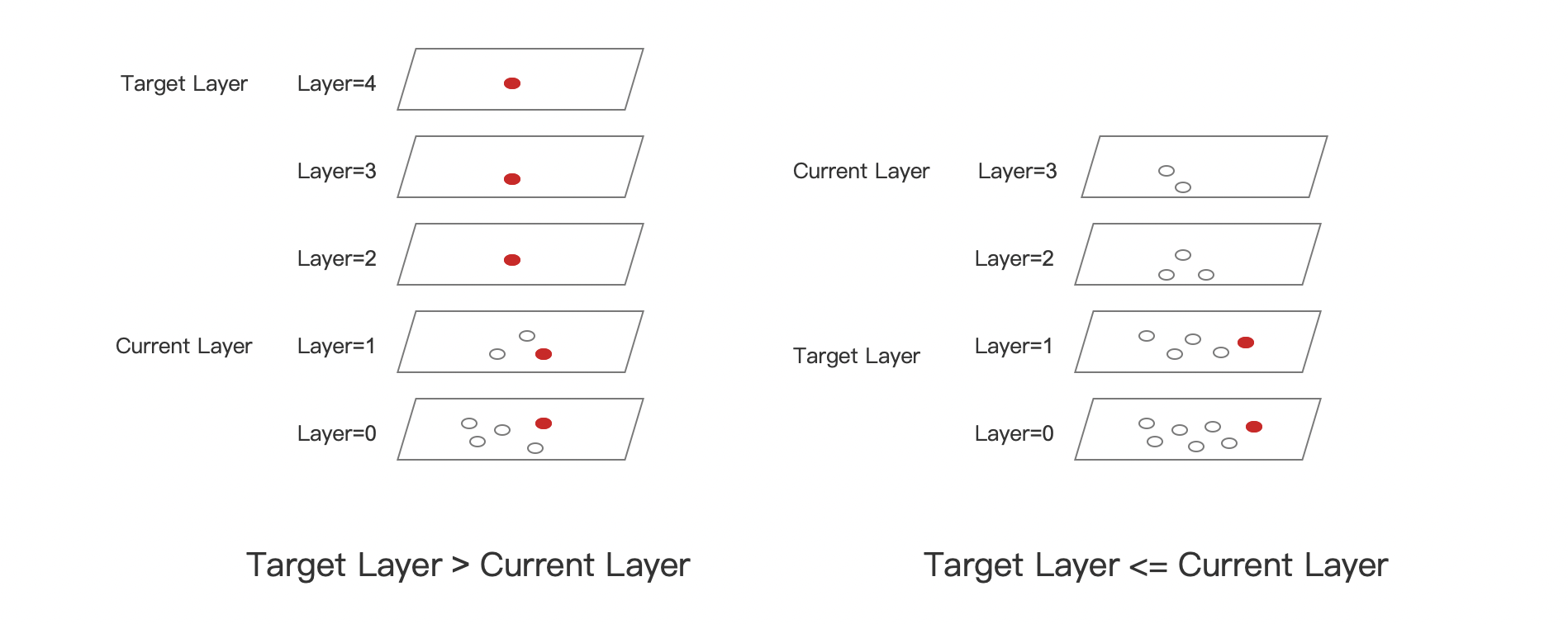
Obtaining layer entry nodes can be summarized in two scenarios, as shown below:

Figure 7：

• Target Layer > Current Layer (highest layer in the graph): In layers 4, 3, and 2, the addition of the new node introduces new layers, so the new node can be directly added to these layers. There is no need to consider the entry node in these cases; in layers 1 and 0, the approach is the same as the other scenario described below.

• Target Layer <= Current Layer: Before reaching the target layer, we need to start from the highest layer and obtain the entry node for each layer, descending layer by layer.

  • Layer 3: As it is the highest layer, the global entry node serves as the entry node for this layer. Finding the candidate neighbors for the new node in this layer , and the Top1 node (called ep3) from the candidate neighbor collectionis selected as the entry node for layer 2.
  • Layer 2: ep3 serves as the entry node for this layer, and the process of finding candidate neighbors for the new node and selecting the Top1 node (called ep2) as the entry node for layer 1.
  • Layer 1: ep2 serves as the entry node, and the process of finding candidate neighbors for the new node and the TopK node collection (called ep1) from the candidate neighbors is selected as the entry nodes for layer 0.
  • Layer 0: The node collection named ep1 serves as the entry nodes for this layer.

  It is worth noting that in layers 1 and 2, only the Top1 (closest neighbor) from the previous layer’s neighbor collection is used as the entry node, while in layer 0, a collection of TopK nodes is selected. The rationale behind this is to balance the needs for search efficiency and accuracy:

  • Choosing the closest neighbor as entry node: This focuses on quickly narrowing down the search area and getting as close as possible to the target node.
  • Using multiple neighbors as entry node: This improves the comprehensiveness of the search, especially in complex or high-dimensional data spaces. Using multiple entry nodes allows exploring the space from different paths, increasing the chances of finding the best match.

Why Descend Layer by Layer Instead of Directly Reaching the Target Level

In Figure 7 notice that, when Target Layer <= Current Layer, the approach is to descend layer by layer rather than starting directly from the target level. The considerations include:

• Fast Navigation in Higher Layers: In higher layers, the connections between nodes cover larger distances. This means that searching in higher layers can quickly skip irrelevant areas and rapidly approach the target area of the new node. Jumping directly to the target layer might miss this opportunity for rapid approach.
• Gradually Refining the Search: Starting from higher layers and descending layer by layer allows the search process to become progressively more refined. In each layer, the search adjusts its direction according to the connection structure of that layer, approaching the position of the new node more precisely. This layered refinement process helps in finding a more accurate nearest neighbor.
• Avoiding Local Minima: Direct searching in the target layer could result in falling into local minima, where the nearest neighbor found is not the closest neighbor globally. Descending layer by layer helps avoid this as each layer’s search is based on the results of the previous layer, offering a more comprehensive perspective.
• Balancing Search Costs: While descending layer by layer might seem more time-consuming than jumping directly to the target layer, it is often more efficient. This is because fewer search steps are needed in higher layers, whereas direct searching in the denser lower layers might require more steps to find the nearest neighbor.

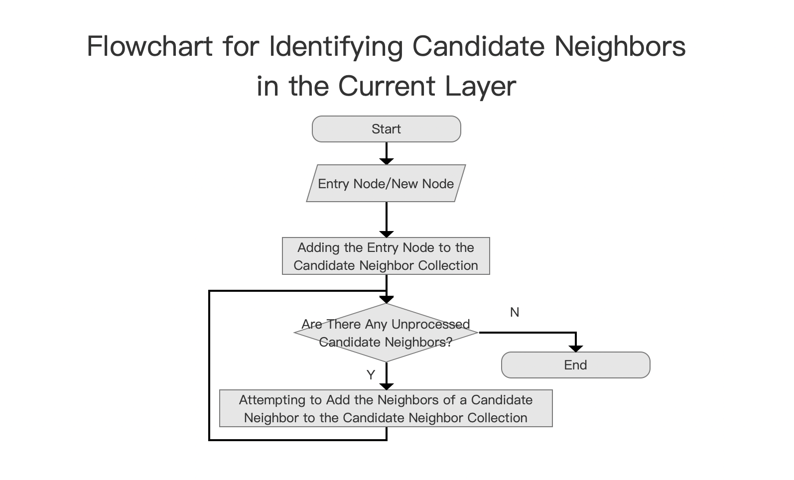
Identifying Candidate Neighbors in the Current Layer

Figure 8：

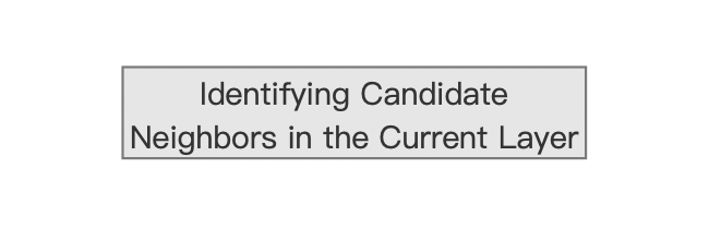
Identifying candidate neighbors in the current layer is a search process of a greedy algorithm. It starts from the entry node, initially considering it as the node that seems closest to the new node. If a node’s neighbor appears closer to the newly inserted node, the algorithm shifts to that neighbor and continues exploring its neighbors. Eventually, it finds the TopN closest nodes (note that these TopN nodes may not necessarily be the closest to the new node). The flowchart is as follows:

Figure 9：

Candidate Neighbor Collection

The data structure for the candidate node collection is a min-heap, sorted by node distance scores, with closer distances receiving higher scores. Node distance refers to the distance between the new node and the candidate neighbors.

Key Points in the Greedy Algorithm’s Search Process

• Distance Score Threshold: During the search process, a threshold called minCompetitiveSimilarity is continuously updated, which is the top element of the min-heap. If the distance between a neighbor and the new node is less than this threshold, nodes connected to this neighbor are no longer processed.
• Recording Visited Nodes: Due to the interconnections between nodes, the greedy algorithm can easily revisit the same nodes. Recording visited nodes improves search performance.
• Entry Node for the Next Layer: The TopN from the candidate neighbor collection of the current layer will serve as the entry nodes for the next layer, as mentioned above, the Top1 and TopK (here, K is defined in the source code by a variable named beamWidth, with a default value of 100).

Close Enough Neighbors vs. Absolute Closest Neighbors

The greedy algorithm’s search process means that it might not find the absolute closest neighbors but usually finds neighbors close enough:

• The algorithm’s goal is to find neighbors close enough to the new node. Here, “close enough” means that while the neighbors found may not be the absolute closest (i.e., some nodes closer to the new node are not chosen as neighbors), they are sufficiently close to effectively represent the new node’s position in the graph.
• Efficiency and Accuracy Balance: In practical applications, finding the absolute closest neighbors can be very time-consuming, especially in large-scale or high-dimensional datasets. Therefore, the algorithm often seeks a balance point, finding close enough neighbors within an acceptable computational cost.
• Greedy Search Strategy: HNSW uses a greedy algorithm to progressively approximate the nearest neighbors of the new node. This means that at each step, the algorithm chooses the neighbor that currently appears closest to the new node. This method usually finds close enough neighbors quickly but does not always guarantee finding the absolute closest neighbors.
• Practical Considerations: In most cases, finding “close enough” neighbors meets the needs of most application scenarios, such as approximate nearest neighbor search. This approach ensures search efficiency while providing relatively high search accuracy.
• Limiting Neighbor Numbers: To control the complexity of the graph, the number of neighbors for each node is usually limited. This means that even if closer nodes exist, they might not be chosen as neighbors of the new node due to the limit on the number of neighbors.

Selecting Candidate Neighbors Based on Diversity

Figure 10：

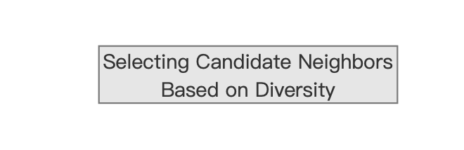
Although we have already found the TopN “close enough” neighbors in the previous step, Identifying Candidate Neighbors in the Current Layer, we still need to examine these neighbors for diversity based on the following factors. Neighbors that do not meet the diversity criteria will not be connected, and diversity checking is achieved by calculating the distances between neighbors:

• Covering Different Areas: If the neighbors of a node are far apart from each other, it means they cover different areas around the node. This distribution helps quickly locate different areas during the search process, thereby improving search efficiency and accuracy.
• Avoiding Local Minima: In high-dimensional spaces, if all neighbors are very close, the search process may fall into local minima, where the nearest neighbor found is not the closest globally. Distance differences between neighbors provide more search paths to avoid this situation.
• Enhancing Graph Connectivity: Neighbors with distance differences can enhance the connectivity of the graph, making the paths from one node to another more diverse. This is important for quickly propagating information or finding optimal paths in the graph.
• Adapting to Different Data Distributions: In real applications, data is often not uniformly distributed. Ensuring distance differences between neighbors can better adapt to these non-uniform data distributions, ensuring the graph structure effectively covers the entire data space.
• Balancing Exploration and Exploitation: In search algorithms, there needs to be a balance between exploration (exploring unknown areas) and exploitation (using known information). Distance differences between neighbors help this balance, as it allows the algorithm to explore multiple directions from a node, rather than being limited to the closest neighbors.
• Improving Robustness: In dynamically changing datasets, the distribution of data points may change over time. If a node’s neighbors have a certain distance difference, this helps the graph structure adapt to these changes, maintaining its search efficiency.

Diversity Check

The checking process flowchart is as follows:

Figure 11：

Neighbor Collection

The elements in the neighbor collection are N nodes selected from the candidate neighbor collection after diversity checking, and they will become the official neighbors of the new node.

Note that in layer 0, a node can connect to up to 2*maxConn neighbor nodes, while in other layers, it can connect to a maximum of maxConn nodes, which is the size of the neighbor collection. The default value of maxConn is 16.

In the source code, the NeighborArray object represents a node’s neighbor information:

Figure 12：

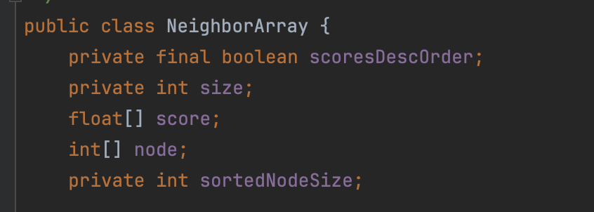
• size: The number of neighbors
• score: An array of distance scores between the node and its neighbors
• node: An array of neighbor node identifiers
• scoresDescOrder: Whether the node and score arrays are sorted in ascending or descending order by distance score
• sortedNodeSize: This is not relevant for this article

Sorting the Candidate Neighbor Collection

As mentioned earlier, the candidate neighbor collection is a min-heap, with the top element being the farthest distance. Since the subsequent flow Does the Neighbor Node Meet the Diversity Criteria?? requires starting from the closest (highest score), the Sorting the Candidate Neighbor Collection in the source code involves writing the heap elements into a NeighborArray called scratch, sorted in ascending order by distance score.

Checking Each Candidate Neighbor for Diversity

Starting with the highest scored element in scratch, compare its distance with each neighbor in the neighbor collection d(neighbor, new node's other neighbors). If there is at least one other neighbor such that d(neighbor, new node) is less than d(neighbor, new node's other neighbors), it does not meet diversity. If it meets diversity, add this candidate neighbor node to the neighbor collection; it will become an official neighbor of the new node in that layer.

Attempting to Add the New Node as a New Neighbor of Its Neighbors

图13：

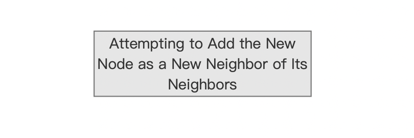
This process point is closely related to the graph’s update strategy. When a new node is added to the graph, it is necessary to update the graph structure according to specific rules or strategies. This includes which nodes should be included in the new node’s neighbor list, as discussed above, and deciding which existing nodes should add the new node to their neighbor lists. These update strategies typically consider the following aspects:

• Maintaining Graph Connectivity: The update strategy aims to maintain good connectivity of the graph, ensuring effective navigation from any node to others.
• Optimizing Search Efficiency: By appropriately updating neighbor lists, the structure of the graph can be optimized, thereby improving the efficiency of subsequent search operations.
• Maintaining Neighbor Diversity: Update strategies often aim to maintain diversity among neighbors, which helps to enhance the comprehensiveness and accuracy of searches.
• Controlling Graph Size and Complexity: To avoid making the graph overly complex, update strategies may include limiting the maximum number of neighbors for a node.
• Adapting to Data Changes: In dynamically changing datasets, update strategies help the graph adapt to the addition of new data, maintaining its ability to reflect the current state of the dataset.

图14：

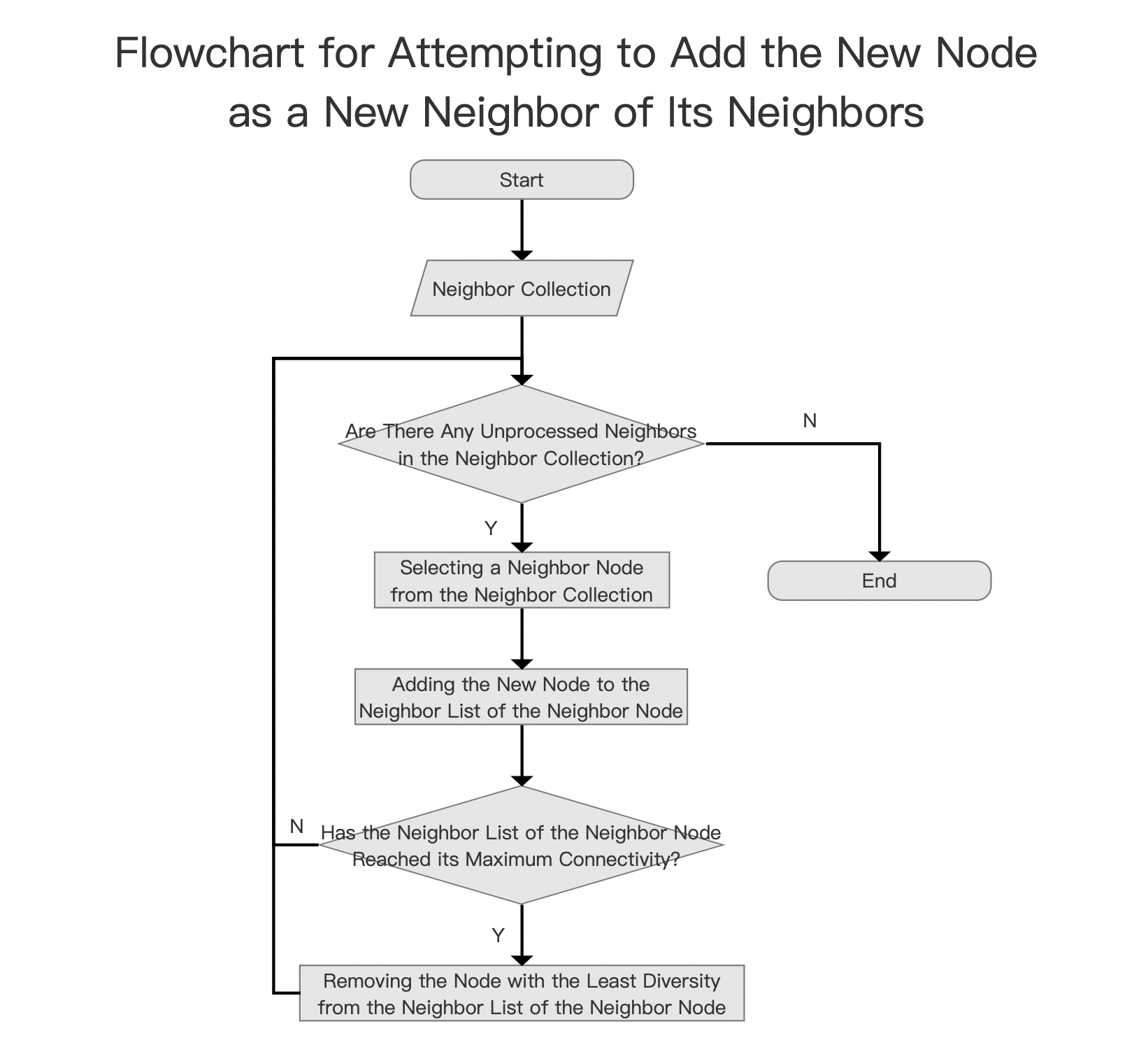
The neighbor collection contains the new node’s official neighbors, and a unidirectional connection has already been established with them. If the neighbor’s neighbor list of the new node has not yet reached the connection limit, i.e., 2*maxConn in layer 0 and maxConn in other layers, then the new node can be added as a neighbor of its neighbor. Otherwise, after being added to the neighbor’s neighbor list, a diversity check is performed (following the same logic as described earlier), and the node with the least diversity is removed from the list. Of course, this least diverse node might be the new node or some other node in the list.

Conclusion

  This article outlines the process of constructing an HNSW graph in Lucene 9.8.0, and the subsequent graph data will be stored using index files . However, currently, this article is only available in Chinese.